Background

As part of my Intermediate Macroeconomics class, I was tasked with analyzing a concept covered in class using real world data. I decided to do an anaylsis on whether Okun’s Law (a theory stating there is an inverse relation between real GDP growth and the unemployment rate) has held true in the United States since 2000 (because it hasn’t at some times, like the Oil Crisis of the 1970s) by creating a graph in Python to make it easier to understand the data.

Process

I started off by locating the datasets at the St. Louis Federal Reserve Bank’s FRED, and then used an API to simplify the data collection process, creating a dataframe for unemployment and GDP data.

from fredapi import Fred
import pandas as pd
import seaborn as sns
import matplotlib.pyplot as plt

fred = Fred(api_key='')

# Get data for real GDP
gdp_data = fred.get_series('GDPC1')
gdp_df = gdp_data.reset_index()
gdp_df.columns = ["Date", "GDP"]

# Get data for unemployment rate
unemployment_data = fred.get_series('UNRATE')
unemployment_df = unemployment_data.reset_index()
unemployment_df.columns = ["Date", "Unemployment Rate"]

With the data in hand, I began to prepare the data, first by merging my two datasets into one and selecting only the data beginning in 2000, since the it went as far back as the 1940s. Then I calculated the percentage change for GDP and the difference in the unemployment rate, both changing quarterly, and placed these into their respective columns.

# Merge unemployment rate and GDP data into one dataframe and select data since 2000
okun_law_df = pd.merge(gdp_df, unemployment_df, on=['Date'])
okun_law_df = okun_law_df.loc[(okun_law_df['Date'].dt.year >= 2000) & (okun_law_df['Date'].dt.month >= 1)]

# Get percentage change for GDP and difference for unemployment rate
okun_law_df['Percentage Change in GDP'] = (okun_law_df['GDP'].pct_change())*100
okun_law_df['Change in Unemployment Rate'] = okun_law_df['Unemployment Rate'].diff()

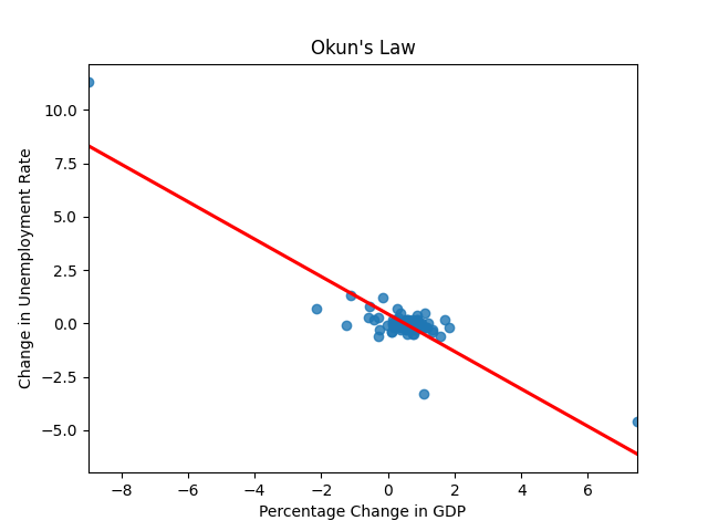
Lastly, I created the plot, a scatterplot with a trendline to best show the data in an easy to understand format.

# Create and show plot
sns.regplot(x='Percentage Change in GDP', y='Change in Unemployment Rate',
            data=okun_law_df, ci=None,
            line_kws={'color':'red'}).set(title="Okun's Law")
plt.show()

The final result:

Analysis and Conclusion

With most of the data points being clustered around (0, 0), we can see that there wasn’t much of a change quarter to quarter since 2000, with the two noticeable exceptions of (-9.0, 11.3), for April 1, 2020, and (7.5, -4.6), for July 1, 2020. These show the initial effects of the COVID-19 pandemic, a massive decrease in real GDP and increase in the unemployment rate, and the quick economic recovery, with real GDP almost returning to prepandemic levels and the unemployment rate making huge strides in its recovery. There were a few data points that were not in line with Okun’s Law. For example, the data points (0.9, 0.4), for January 1, 2001, and (1.1, 0.5), for October 1, 2009, show a simultaneous increase in real GDP and the unemployment rate. To get a more certain answer, I also calculated the correlation coefficient to be -0.88, signifying a very strong inverse association between the two variables. This meaning that Okun’s Law has held true since 2000.